Atan2

atan2（アークタンジェント2）は、関数の一種。「2つの引数を取るarctan（アークタンジェント）」という意味である。x軸の正の向きと、点(x, y) （ただし、(0, 0)ではない）まで伸ばした半直線（レイ）との間の、ユークリッド平面上における角度として定義される。関数は${\displaystyle \operatorname {atan2} (y,x)}$もしくは${\displaystyle \operatorname {arctan2} (y,x)}$の形をとり、値はラジアンで返ってくる。

関数${\displaystyle \operatorname {atan2} (y,x)}$は、プログラミング言語のFortran（IBM社が1961年に実装したFORTRAN-IV）において最初に登場した。元々は、角度θを直交座標系の(x, y)から極座標系の(r, θ)に変換する際に、正確で一意な値が返ってくることを意図して導入された。また、${\displaystyle \operatorname {atan2} (y,x)}$は複素数${\displaystyle x+iy}$の偏角^{[注釈 1]}を求める際にも利用される。

関数${\displaystyle \operatorname {atan2} (y,x)}$ は、−π < θ ≤ πの範囲で、

${\displaystyle {\begin{aligned}x&=r\cos \theta \\y&=r\sin \theta \end{aligned}}}$

（ただし、r > 0）となる単一の値θを返す。

なお、arctanを使って角度θを求める際に注意すべきことであるが、${\displaystyle r={\sqrt {x^{2}+y^{2}}}}$が真であるからと言って、

${\displaystyle \theta =\arctan \left({\frac {y}{x}}\right)}$

であるということが常に言えるとは限らない。

これは、x > 0だった場合にのみ当てはまる。もしx < 0だった場合は、上の式から導出された角度は、正しい角度とは正反対の方向を指し示している。そして、デカルト点(x, y)をユークリッド平面上の正しい象限に配置するには、${\displaystyle \pi }$（度数法で言うと180°）の値をθに加算または減算する必要がある^[1]。これはつまり、正しい角度を出すためにはxおよびyの符号の情報がそれぞれ別個に必要とされると言うことであり、もし単にyをxで除算した場合は、その情報が失われてしまうというわけである。その点、atan2は細かいことを気にしなくてもyとxに代入すれば普通に正しい角度を返してくれるので便利である。

関数${\displaystyle \operatorname {atan2} (y,x)}$の戻り値である角度θについては、xとyの値を変更しないままでも角度θに2πの任意の整数倍を加算することが可能であるため、つまり区間をちゃんと設定しないと戻り値の値が曖昧になってしまうため、関数atan2はその主値として、区間を(−π, π)としたものが戻り値として返ってくるようになっている（関数arctanの戻り値の区間が(−π/2 , π/2)である点との違いに注意）。角度θ は符号付き角度であり、反時計回りの角度は正、時計回りは負となる。具体的に言うと、もしy ≥ 0だった場合は[0, π] の区間にあり、もしy < 0だった場合には(−π, 0)の区間にある、と言う感じになるように関数${\displaystyle \operatorname {atan2} (y,x)}$の内部で場合分けをしている。

atan2が生み出された経緯と動機

atan2関数は、元々は特定のプログラミング言語に実装された関数（サブルーチン）の一つに過ぎなかったが、現在では他の科学技術の分野でもよく使われるものとなっている。その起源は少なくとも、古のプログラミング言語であるFORTRANのATAN2(Y, X)にまで遡ることができるが^[2]、現在^[いつ?]においては他の現代的なプログラミング言語にも標準的な数学関数ライブラリやパッケージの形で実装されている。例を挙げると、C言語およびC++の標準ライブラリ（標準Cライブラリのmath.hにおけるatan2()関数あるいは標準C++ライブラリのcmathにおけるstd::atan2()関数）、Javaの標準ライブラリにおけるMath.atan2()メソッド、C#/F#/VB.NETなどから利用できる.NETの基本クラスライブラリにおけるSystem.Math.Atan2()メソッド^[3]、JavaScriptの標準組み込みオブジェクトMath、Pythonのmathモジュール、RubyのMathモジュール、Goのmathパッケージ^[4]、などであるが、他にも多数の言語に実装されている。さらに言うと、Perlを始めとする古いスクリプト言語にも、C言語風のatan2(y, x)関数が実装されていることが多い。

atan2関数が生み出された背景として、単一引数のみを取るアークタンジェント（arctan関数）は正反対の方向を区別できない、と言う使い勝手の悪さがある。例えば、x軸とベクトル(1, 1)がなす反時計回りの角度を、arctan関数を使って「arctan(1/1)」のような形で計算した場合、「π/4ラジアン（つまり度数法で言うと45°）」という答えが返ってくる。しかし、x軸とベクトル(−1, −1)の間の角度を同様に、「arctan(−1/−1)」のような形で計算してみると、期待される答えは「−3π/4ラジアン(−135°)」または「5π/4ラジアン(225°)」であるにもかかわらず、やっぱり「π/4ラジアン」が返ってくる。arctan関数の使い勝手の悪さをさらに言うと、x軸とベクトル(0, y)(ただし、y ≠ 0とする)がなす角度をarctan関数で計算しようとすると、これはarctan(y/0)の評価が必要になるわけだが、こんなことをさせるとコンピューターはゼロ除算のエラーを吐いてバグる。^[要校閲]

atan2関数は、2つの変数 y と xから一意なアークタンジェントの値を算出するが、そのとき両変数の正負の符号が、実行結果の象限を決定するために利用される。それに基づいて、アークタンジェントで「y/x」したときの結果の中から、求める値が出るような分岐先に飛ばしている。例を挙げると、「atan2(1, 1) = π/4」 と 「atan2(−1, −1) = −3π/4」のどちらに分岐するのか、と言ったことを判別している。また、例えば「ゼロ除算のエラーを吐いてバグる」の代わりに「atan2(1, 0) = π/2」に分岐させるときも、同様の方法で飛ばしている。^[要校閲]

もちろん、場合によって必要な象限補正と例外処理をいちいち精査することで、上記の計算を力技で行うことは可能だが、そんなことをするよりも、常に一意な正しい結果を返してくれるような1つの関数が存在した方が便利である。そんな経緯でatan2関数が存在する。atan2関数は様々な応用（アプリケーション）において有用であり、例えばユークリッド空間上におけるユークリッド点に関して、1つの点から別の点へと至る方向ベクトルを調べるのに便利である。主な用途としては、コンピューターグラフィックス（CG）における回転において、回転行列をオイラー角に変換する際に使われる。^[要校閲]

定義と計算

定義

関数 atan2 は複素数 x + yi に偏角関数 arg を適用した時の主値を計算する。すなわち、atan2(y, x) = Pr arg(x + yi) = Arg(x + yi) である。偏角は、2π（原点を中心としたちょうど1周の回転に対応）の整数倍を加えたものも同じ角度になるが、atan2 を一意に定義するために範囲 ${\displaystyle (-\pi ,\pi ]}$ の主値を使用する。つまり、−π < atan2(y, x) ≤ π とする。

標準の arctan 関数（値域 (−π/2, π/2)）を用いて、次のように表すことができる:

${\displaystyle \operatorname {atan2} (y,x)={\begin{cases}\arctan({\frac {y}{x}})&{\text{if }}x>0,\\\arctan({\frac {y}{x}})+\pi &{\text{if }}x<0{\text{ and }}y\geq 0,\\\arctan({\frac {y}{x}})-\pi &{\text{if }}x<0{\text{ and }}y<0,\\+{\frac {\pi }{2}}&{\text{if }}x=0{\text{ and }}y>0,\\-{\frac {\pi }{2}}&{\text{if }}x=0{\text{ and }}y<0,\\{\text{undefined}}&{\text{if }}x=0{\text{ and }}y=0.\end{cases}}}$

重複する4つの半平面を用いたコンパクトな式:

${\displaystyle \operatorname {atan2} (y,x)={\begin{cases}\arctan \left({\frac {y}{x}}\right)&{\text{if }}x>0,\\{\frac {\pi }{2}}-\arctan \left({\frac {x}{y}}\right)&{\text{if }}y>0,\\-{\frac {\pi }{2}}-\arctan \left({\frac {x}{y}}\right)&{\text{if }}y<0,\\\arctan \left({\frac {y}{x}}\right)\pm \pi &{\text{if }}x<0,\\{\text{undefined}}&{\text{if }}x=0{\text{ and }}y=0.\end{cases}}}$

アイバーソンの記法を用いれば、さらにコンパクトな式が可能:

${\displaystyle \operatorname {atan2} (y,x)}$	${\displaystyle =\arctan \left({\frac {y}{x}}\right)[x\neq 0]+\operatorname {sgn}(y)\left(\pi [x<0]+{\frac {\pi }{2}}[x=0]\right)}$
	${\displaystyle +\;{\text{undefined}}\;\![x=0\wedge y=0]}$ [注釈 2]

一見すると条件式のない数式:

${\displaystyle \operatorname {atan2} (y,x)=\operatorname {sgn}(x)^{2}\arctan \left({\frac {y}{x}}\right)+{\frac {1-\operatorname {sgn}(x)}{2}}\left(1+\operatorname {sgn}(y)-\operatorname {sgn}(y)^{2}\right)\pi }$

タンジェントの半角の公式から派生した次の式で atan2 を定義することもできる:

${\displaystyle \operatorname {atan2} (y,x)={\begin{cases}2\arctan \left({\frac {y}{{\sqrt {x^{2}+y^{2}}}+x}}\right)&{\text{if }}x>0{\text{ or }}y\neq 0,\\\pi &{\text{if }}x<0{\text{ and }}y=0,\\{\text{undefined}}&{\text{if }}x=0{\text{ and }}y=0.\end{cases}}}$

この式は、上記の定義よりもシンボリックな使用に適している場合がある。ただし、${\displaystyle {\sqrt {x^{2}+y^{2}}}}$ の丸め誤差の影響が領域 x < 0, y = 0 の近くで拡大するため、一般的な浮動小数点数の計算用途には適していない（これにより、yがゼロで除算されることもある）。

これらの膨らんだ丸め誤差を回避するため、先ほどの式を変形:

${\displaystyle \operatorname {atan2} (y,x)={\begin{cases}2\arctan \left({\frac {y}{{\sqrt {x^{2}+y^{2}}}+x}}\right)&{\text{if }}x>0,\\2\arctan \left({\frac {{\sqrt {x^{2}+y^{2}}}-x}{y}}\right)&{\text{if }}x\leq 0{\text{ and }}y\neq 0,\\\pi &{\text{if }}x<0{\text{ and }}y=0,\\{\text{undefined}}&{\text{if }}x=0{\text{ and }}y=0.\end{cases}}}$

注意:

• これにより、範囲 (−π, π] の結果が生成される。^{[注釈 3]}
• 上記のように、偏角の主値 atan2(y, x) は、三角法によって arctan(y/x) に関連付けることができる。 導出は次のようになる:

(x, y) = (r cos θ, r sin θ) のとき tan(θ/2) = y / (r + x) となる。その結果、次式が成立する。

${\displaystyle {\text{atan2}}(y,x)=\theta =2\,\theta /2=2\arctan {\frac {y}{{\sqrt {x^{2}+y^{2}}}+x}}.}$

問題の領域は √x² + y² + x ≠ 0 であることに注意。

微分

関数 atan2 は2変数関数であるため、2つの偏導関数がある。これらの導関数が存在する点では、atan2 は定数項を除いた arctan(y/x) に等しくなる。したがって、x > 0 または y ≠ 0 の場合、

${\displaystyle {\begin{aligned}&{\frac {\partial }{\partial x}}\operatorname {atan2} (y,\,x)={\frac {\partial }{\partial x}}\arctan \left({\frac {y}{x}}\right)=-{\frac {y}{x^{2}+y^{2}}},\\[5pt]&{\frac {\partial }{\partial y}}\operatorname {atan2} (y,\,x)={\frac {\partial }{\partial y}}\arctan \left({\frac {y}{x}}\right)={\frac {x}{x^{2}+y^{2}}}.\end{aligned}}}$

したがって、atan2 の勾配は次式で与えられる。

${\displaystyle \nabla {\text{atan2}}(y,x)=\left({-y \over x^{2}+y^{2}},\ {x \over x^{2}+y^{2}}\right).}$

関数 atan2 を角度関数 θ(x, y) = atan2(y, x) （定数を除いて定義）として省略して表すと、全微分について次の式が得られる:

${\displaystyle {\begin{aligned}\mathrm {d} \theta &={\frac {\partial }{\partial x}}\operatorname {atan2} (y,\,x)\,\mathrm {d} x+{\frac {\partial }{\partial y}}\operatorname {atan2} (y,\,x)\,\mathrm {d} y\\[5pt]&=-{\frac {y}{x^{2}+y^{2}}}\,\mathrm {d} x+{\frac {x}{x^{2}+y^{2}}}\,\mathrm {d} y.\end{aligned}}}$

関数 atan2 は、負の x 軸に沿って不連続であるが、角度を連続的に定義できないという事実を反映して、この導関数は原点を除いて連続的に定義される。これは、角度の微小な（そして実際には局所的な）変化が原点を除くすべての場所で定義できるという事実を反映している。この導関数をパスに沿って積分するとパス全体の角度が全体的に変化し、閉ループで積分すると回転数が得られる。

微分幾何学の言語では、この導関数は1-形式であり、閉である（導関数が0である）が、完全ではない（0-形式の導関数、つまり関数ではない）。実際、1点を除いた平面（Punctured Plane）の1次のド・ラームコホモロジーを生成する。これはそのような形式の最も基本的な例であり、微分幾何学の基本である。

atan2 の偏導関数には三角関数が含まれていないため、三角関数の評価にコストがかかる可能性がある多くのアプリケーション（例：組み込みシステム）で特に役立つ。

図による可視化

この図は、ある半直線に沿ったatan2の値を単位円上に示している。atan2の値はラジアンであり、単位円内に記載されている。標準的な数学の方式に従い、角度は右方向の半直線をゼロとして反時計回りに増加する。ここで、2つの引数の順序が座標と比べて入れ替わっていることに注意が必要である。すなわち、関数atan2(y, x)は座標(x, y)に対応する角度を計算する。

この図は${\displaystyle \arctan(\tan(\theta ))}$と、${\displaystyle 0\leq \theta \leq 2\pi }$におけるの${\displaystyle \operatorname {atan2} (\sin(\theta ),\cos(\theta ))}$値を示している。両方の関数ともに奇関数であり、それぞれ${\displaystyle \pi }$と${\displaystyle 2\pi }$の周期関数である。このため、${\displaystyle \theta }$の実数値における補角となることが出来る。一例として${\displaystyle \operatorname {atan2} }$の${\displaystyle \theta =\pi }$における分岐截断、および${\displaystyle \arctan }$の${\displaystyle \theta \in \{{\tfrac {\pi }{2}},\;{\tfrac {3\pi }{2}}\}}$における分岐截断が明確に確認出来る。^[5]

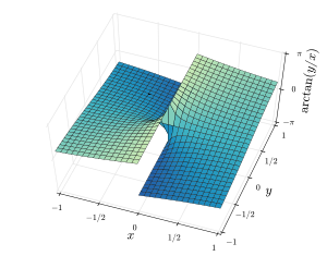
下記の2つの図は、atan2(y, x)およびarctan(y/x)の上から見た3次元図である。ここで、atan2(y, x)におけるX/Y平面の原点から伸びる半直線が定数値なのに対し、arctan(y/x)ではX/Y平面の原点を通る直線が定数値である。x > 0において、2つの図は同一の値となる。

加法定理

${\displaystyle \operatorname {atan2} }$の和は、下記の定理によれば1つの式にまとめることができる。

${\displaystyle \operatorname {atan2} (y_{1},x_{1})\pm \operatorname {atan2} (y_{2},x_{2})=\operatorname {atan2} (y_{1}x_{2}\pm y_{2}x_{1},x_{1}x_{2}\mp y_{1}y_{2})}$

...ここで${\displaystyle \operatorname {atan2} (y_{1},x_{1})\pm \operatorname {atan2} (y_{2},x_{2})\in (-\pi ,\pi ]}$.

証明には、${\displaystyle y_{2}\neq 0}$ または ${\displaystyle x_{2}>0}$、および${\displaystyle y_{2}=0}$ かつ ${\displaystyle x_{2}<0}$の二つのケースにわけて行う必要がある。 ここでは前者の${\displaystyle y_{2}\neq 0}$ または ${\displaystyle x_{2}>0}$のケースのみにおいて考える。最初に、下記の考察を行う：

1. ${\displaystyle -\operatorname {atan2} (y,x)=\operatorname {atan2} (-y,x)}$ において ${\displaystyle y\neq 0}$ または ${\displaystyle x>0}$.
2. ${\displaystyle \operatorname {Arg} (x+iy)=\operatorname {atan2} (y,x)}$であり、${\displaystyle \operatorname {Arg} }$は複素数の偏角の数値計算である。
3. ${\displaystyle \theta \in (-\pi ,\pi ]}$である限り、${\displaystyle \theta =\operatorname {Arg} e^{i\theta }}$が成り立つ（オイラーの公式により）。
4. ${\displaystyle \operatorname {Arg} (e^{i\operatorname {Arg} \zeta _{1}}e^{i\operatorname {Arg} \zeta _{2}})=\operatorname {Arg} (\zeta _{1}\zeta _{2})}$.

(4)において、複素数の偏角の定理により${\displaystyle e^{i\operatorname {Arg} \zeta }={\bar {\zeta }}}$、ここで ${\displaystyle {\bar {\zeta }}=\zeta /\left|\zeta \right|}$、従って ${\displaystyle \operatorname {Arg} (e^{i\operatorname {Arg} \zeta _{1}}e^{i\operatorname {Arg} \zeta _{2}})=\operatorname {Arg} ({\bar {\zeta _{1}}}{\bar {\zeta _{2}}})}$となる。さらに、全ての正の実数値${\displaystyle a}$に対して${\displaystyle \operatorname {Arg} \zeta =\operatorname {Arg} a\zeta }$が成り立ち、${\displaystyle \zeta =\zeta _{1}\zeta _{2}}$ および ${\displaystyle a={\frac {1}{\left|\zeta _{1}\right|\left|\zeta _{2}\right|}}}$ とすると、${\displaystyle \operatorname {Arg} ({\bar {\zeta _{1}}}{\bar {\zeta _{2}}})=\operatorname {Arg} (\zeta _{1}\zeta _{2})}$となる。

上記より、次の等式が成り立つ：

${\displaystyle {\begin{aligned}\operatorname {atan2} (y_{1},x_{1})\pm \operatorname {atan2} (y_{2},x_{2})&{}=\operatorname {atan2} (y_{1},x_{1})+\operatorname {atan2} (\pm y_{2},x_{2})&{\text{by (1)}}\\&{}=\operatorname {Arg} (x_{1}+iy_{1})+\operatorname {Arg} (x_{2}\pm iy_{2})&{\text{by (2)}}\\&{}=\operatorname {Arg} e^{i(\operatorname {Arg} (x_{1}+iy_{1})+\operatorname {Arg} (x_{2}\pm iy_{2}))}&{\text{by (3)}}\\&{}=\operatorname {Arg} (e^{i\operatorname {Arg} (x_{1}+iy_{1})}e^{i\operatorname {Arg} (x_{2}\pm iy_{2})})\\&{}=\operatorname {Arg} ((x_{1}+iy_{1})(x_{2}\pm iy_{2}))&{\text{by (4)}}\\&{}=\operatorname {Arg} (x_{1}x_{2}\mp y_{1}y_{2}+i(y_{1}x_{2}\pm y_{2}x_{1}))\\&{}=\operatorname {atan2} (y_{1}x_{2}\pm y_{2}x_{1},x_{1}x_{2}\mp y_{1}y_{2})&{\text{by (2)}}\end{aligned}}}$

Corollary（推論）: もし ${\displaystyle (y_{1},x_{1})}$ および ${\displaystyle (y_{2},x_{2})}$ が2次元のベクトルであり、これらベクトル間の角度を計算するのに ${\displaystyle \operatorname {atan2} }$を用いた差分の式が頻繁に用いられているとすると、計算結果は${\displaystyle (-\pi ,\pi ]}$の区間となることから、ほとんどのケースではレンジチェックは不要となる。

東-反時計回り、北-時計回り および 南-時計回り等の変換

${\displaystyle \mathrm {atan2} }$関数は元々数学的に多く用いられる、原点から右の半直線から反時計回りに動く場合の変化について定義している（ここではこれを東-反時計回りと言う）。一方実際の実装系では、北-時計回り および 南-時計回りの変換がよく用いられる。 例えば気象学において、風向は${\displaystyle \mathrm {atan2} }$関数を用いて、風の東および北向きの成分を引数として利用して計算されている。^[6] 同様に太陽の方位角（英語版）も東および北方向の成分を引数として用いている。風向きは通常北-時計回りで定義されているためであり、太陽の方位角は北-時計回り および 南-時計回り両方を用いて広く計算されていためである。^[7] これらの異なる変換は、下記のように位置の置換およびx/y座標の符号を下記のように変更することで実現できる：

• ${\displaystyle \mathrm {atan2} (y,x),\;\;\;\;\;}$ (東-反時計回り変換)
• ${\displaystyle \mathrm {atan2} (x,y),\;\;\;\;\;}$ (北-時計回り)
• ${\displaystyle \mathrm {atan2} (-x,-y)}$. (南-時計回り)

例として、${\displaystyle x_{0}={\frac {\sqrt {3}}{2}}}$ で ${\displaystyle y_{0}={\frac {1}{2}}}$の場合、東-反時計回りの場合には${\displaystyle \mathrm {atan2} (y_{0},x_{0})\cdot {\frac {180}{\pi }}=30^{\circ }}$、北-時計回りでは${\displaystyle \mathrm {atan2} (x_{0},y_{0})\cdot {\frac {180}{\pi }}=60^{\circ }}$南-時計回り${\displaystyle \mathrm {atan2} (-x_{0},-y_{0})\cdot {\frac {180}{\pi }}=-120^{\circ }}$のようになる。

x/y成分の符号の変更と位置の転換は結果として８つの${\displaystyle \mathrm {atan2} }$の定義が可能となる。それらは時計回り・反時計回りの４つの方角・東西南北を始点とする。

プログラミング言語における実装

atan2の実装はプログラミング言語ごとに異なる。

• Microsoft Excel^[8]、OpenOffice.org Calc、LibreOffice Calc^[9]、Google Spreadsheets,^[10] iWork Numbers^[11]、およびANSI SQL:2008 standard^[12]では、2つの引数をもつatan2関数はそのままの順序の引数${\displaystyle (\operatorname {Re} ,\operatorname {Im} )}$で定義されている （引数の関係の入れ替わりについては § 図による可視化を参照）。
• MathematicaではArcTan[x, y]の形式が用いられ、引数が一つの場合は通常のアークタンジェントになる。MathematicaではArcTan[0, 0]は不定となる。

入れ替わった順序の引数${\displaystyle (\operatorname {Im} ,\operatorname {Re} )}$は下記で用いられている：

• C言語のatan2関数を始めとする多くのプログラミング言語では、直交座標系から極座標系への変換の手間を減らすため、引数は入れ替わったものが使われており、atan2(0, 0)も定義されている。実装においては−0を除外している、あるいは+0が引数に指定された場合には単純にゼロと定義している。関数は常に[−π, π]の間の値を返し、エラーやNaN (Not a Number)を返すことはしない。
• Common Lispでは引数の数は可変なので、atan関数は1つの場合とx座標を付加した(atan y x)が定義されている。^[13]
• Juliaでは、Common Lispと状況が似ており、atan2の代わりに、1引数形式と2引数形式のatanを持っている^[14]。しかし、コンパイル時のアグレッシブな最適化を可能にするため、Juliaはこの2つ以外にも多数のメソッドを持っている^{[15][注釈 4]}。
• Intelアーキテクチャのx87命令では、 atan2はFPATAN (floating-point partial arctangent) 命令で実装される。^[16]この命令は無限大を扱うことができ、結果は閉区間[−π, π]の値となる。例えば、有限のxに対し、atan2(∞, x) = +π/2となる。特に両方の引数がゼロである時、FPATANは下記のようになる：

  atan2(+0, +0) = +0;

  atan2(+0, −0) = +π;

  atan2(−0, +0) = −0;

  atan2(−0, −0) = −π.

この定義は-0の定義に従ったものとなる。

• コード以外での学術論文などの数学的表記では、通常の arctanおよびtan⁻¹の最初の1文字を大文字にしたArctan^[17]およびTan^−1[18]が用いられる。用法は複素数の偏角と同様で、Atan(y, x) = Arg(x + i y)となる。
• シンボリック算術をサポートする実装系では通常、atan2(0, 0) は不定値あるいはエラーを返す。
• -0、無限大やNaNをサポートする実装系（例：IEEE 754）では、−π and −0を含む値を返すように拡張されている場合がある。これら実装系では、NaNが入力された時にNaNあるいは例外を返すよう実装されていることも多い。
• -0をサポートする実装系（例：IEEE 754)では、atan2(y, x)の実装が−0の入力を的確に処理できない場合、atan2(−0, x), x < 0 の時に−πを返すリスクがある。
• netlibで公開されているフリーの算術ライブラリであるFDLIBM (Freely Distributable LIBM)では、atan2のソースコードが公開されており、IEEEの例外値の対処方法を確認することができる。
• ハードウェアによる乗算器を持たない実装系では、atan2関数はCORDIC（英語版）による数値的に十分な近似により実装されている。よってatan(y)の実装もatan2(y, 1)の実装を用いている場合がある。

関連項目

• hypot（英語版）

脚注

注釈

出典

外部リンク

• ATAN2 Online calculator
• atan2 at Everything2
• PicBasic Pro solution atan2 for a PIC18F

その他のatan2の実装・コード

• Bearing Between Two Points
• Arctan and Polar Coordinates
• What's 'Arccos'?